Large scale modelling
and optimization procedures
A unified algorithmic
approach to modelling and optimization
Resumé. Here are
presented algorithms that combine methods of regression analysis and
optimization algorithms into one set of framework.
The given data. We
supppose here that there is given an N times K matrix X that contains
the technical data. In regression context the rows of X are often
viewed as objects and columns of X as variables. In optimization
context it can be the technical specifications that given in the concrete
situation. The N times M matrix Y is in regression context often
viewed as the response matrix that we want to describe. In optimization
context it often represents the resources that are available. Typically, we
want the solution matrix B not to exceed the available resources Y,
which is formulated as XB£Y.
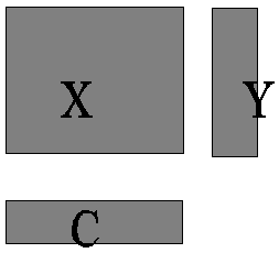
Finally we have the L times K matrix C. In optimization context it can
represent the costs that we want to minimize. In regression context it is
typically an index of quality, environment or costs by which we want to judge
our solution B. Schematically the three matrices X, Y and
C can be shown as follows. It shows that the number of columns of X
and C are the same and also the number of rows of of X and Y.
In regression context we usually do not have the matrix C. We are
typically only interested in finding the solutions B such that XB
describes Y as well as possible.
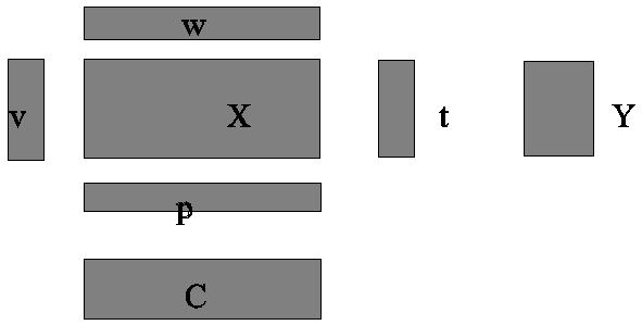
The decomposition of X.
The matrix X is decomposed into rank one parts as follows,
(1) X =
λ1 t1 p1¢
+ λ2 t2 p2¢
+ ...
We call the set (λa
, ta , pa) for components. It is
the set that is selected at each step. The vectors (ta) are
called the score vectors, (pa) the loading
vectors and (λa) scaling constants.
These vectors are determined by certain criteria that reflect the problem in
question. ta is determined by finding a weight vector wa
for the columns of X, and computed as ta=Xwa.
Similarly, the loading vector pa is computed as pa=X¢va,
where va is found by an appropriate criterion. I often use
the language that ta is to describe Y as well as
possible and pa is to report on C as well as
possible. It is clear that there is a symmetry between Y and C.
A criterion used for finding good weight vector wa to use in
computing ta can also be used to find the weight va
for rows of X that is used to compute pa. But usually
there is a different emphasis on C and Y. A typical objective
concerning C is to get as ‘cheap’ solution as possible, because C
represents costs or related terms. The objective concerning Y, on the
other hand, is to obtain a solution B such that XB is ‘close’ to
Y. Thus, the two types of objective can be very different. Also,
although both Y and C are present, the modelling task may be
concerned with only one of them. The role of the different vectors and
matrices are illustrated by the figure below.
The algorithm automatically
computes the generalized inverse, X+, given by
(2) X+
= λ1 r1 s1¢
+ λ2 r2 s2¢
+ ...
This generalized inverse
satisfies XX+X=X. The vectors (ra)
and (sa) satisfy the orthogonality relationships,
ra¢pb=0,
sa¢tb=0,
ra¢pa=1/λa
sa¢ta=1/λa,
a¹b.
The solution B is
computed as B=X+Y. If only A components are
selected, we work with the truncated expression for X and X+
with only the first A terms in (1) and (2).
Requirements to the
solution vector B. We often have certain requirements that the solution B
must satisfy. In fact the algorithm distinguishes between the following
situations:
1) B
can vary freely
2) The
values of B must be non-negative, B³0.
3)
Linear constraints on B. The rows of X are arranged in such a
way that the constaints
are of
following types:
X0B
Free equations
X1B
= Y1 Equality constraints
X2B
£
Y2 Inequality constraints, upper limit
equations
X3B
³
Y3 Inequality constraints, lower limit
equations
Orthogonality. If there
are two objectives in the analysis, i.e., the weight vectors wa
and va are determined according to separate criteria and
independent of each other, neither the score vectors (ta) nor
the loading vectors (pa) will be orthogonal. On the other hand
we get numerially more stable computations, if orthogonality is used. Also, it
is easier to make interpretations there is orthogonality. Therefore, it is often
desirable to make either (ta) or (pa) an
orthogonal set of vectors. If we want orthogonal score vectors we choose the
weight vectors va as va=ta/|ta|.
And similarly, if we want orthogonal loading vectors we choose the weight
vectors wa=pa/|pa|.
Multiplicative criteria of
double objectives. If there is given a criterion to determine wa
and another to determine va, the algorithm uses the product
form of the two criterion. If the two vectors are found independently of each
other, there are no problems. If one of the weight vectors is expressed in terms
od the other one, the algorithm uses a product of the two criteria. Therefore,
it is required to express both criteria as a maximization task. If one criterion
has become very small, only the other criterion is used. E.g., if the squared
covariance is used as a criterion for the weight vector wa and
size of the costs as criterion for va, only the costs
criterion is used, if the squared covariance has reached the zero level.
PLS regression. In PLS
regression the matrix C is not used in the computations. The weight
vector wa is computed as the solution to the eigen system
X¢YY¢X
wa = λ wa.
The criterion that leads to
this is to maximize |Yta|2.
Double PLS regression.
C can be treated in the same way as Y. Thus, we can determine the
weight vector va that maximizes |Cpa|2=|CX¢va|2.
In case we want orthogonal score vectors, we maximize the three terms
a) |CX¢va|2,
b) |Y¢X wa|2
c) |CX¢Xwa|2
|Y¢X wa|2
The wa found
by maximizing c) is used and va=ta/|ta|.
In case a) is small, wa is found by maximizing b). Similarly,
if b) is small, a) is used and if orthogonal score vectors are wanted, the term
maximized is |CX¢Xwa|2.
Linear programming. In
case C is a vector and we want to minimize c¢b
subjet to Xb£y,
b³0, we get
linear programming, where a linear function is minimized subject to linear
constraints. Thus, the algorithm can used to obtain solution to linear
programming tasks. This special way of obtaining the solution follows the PLS
methodology. Thus, the algorithm, the PLS linear programming algorithm,
obtains a balance between the optimization and the associated precision of the
solution. The algorithm identifies the subspace of the columns space of X
that provides with a stable solution. In PLS regression we frequently do not
need many components for appropriate description of Y. In optimization
task we typically need many more components. E.g., if X contains 100 rows
and 200 columns and is densely covered with nonzero values, we may need say 60
components to describe appropriatly the optimal value. In regression context
this is a high value. On the other hand, the exact solution requires 100
components. By working only with 60 components, we get considerably more
stable solution than the exact one.
Organization
of the computations.