Path modeling in linear networks
In many areas of applied sciences and in industrial applications it is known how data blocks are related in time or sequence. It can be instructive to model the data according to this known sequence of the data blocks. There have been developed a large collection of methods to handle this situation. For a review of some introductory analysis see an example.
Topics
| 1. | Introduction. Subdivision of data. |
| 2. | Graphic display of interconnections. |
| 3. | Measures of relationships |
| 4. | The H-method of estimation. One and two data blocks |
| 5. | Three data blocks |
| 6. | Case study |
| 7. | Correlation and prediction |
| 8. | Simple paths |
| 9. | Examples |
| 10. | Comparison of methods |
| 11. | Network of data blocks |
| 12. | Vectors computed (W, T, P, R)i |
| 13. | Regressions among data blocks |
| 14. | Several input (exogenous) and output (endogenous) data blocks |
| 15. | Multiple objectives |
| 16. | Comparisons with overall models |
| 17. | Confidence intervals |
| 18. | Detection of special features |
| 19. | Sensitivity analysis |
| 20. | Case study |
| 21. | Guidelines for presentation of results |
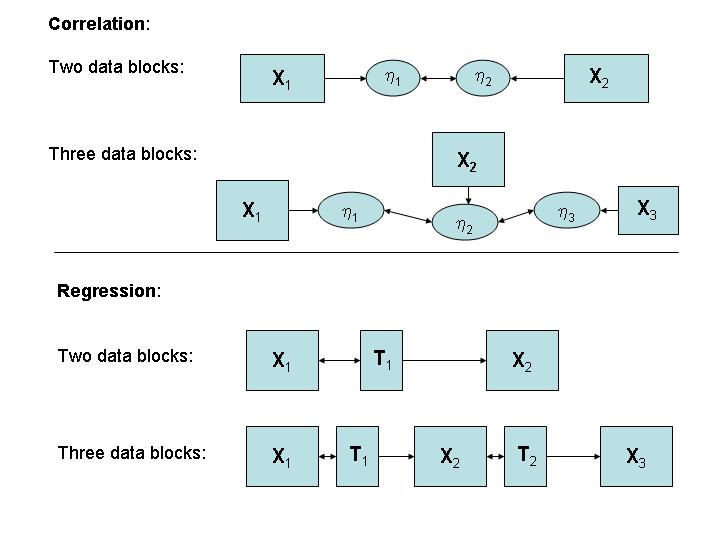
There are two types of approach that are of importance. They are correlation and regression approaches. They are illustrated in the figure below. Consider the case of correlation. If there are two blocks, we are looking for latent variables h1=X1w1 and h2=X2w2 such that latent variables have maximal correlation. In the case of three data bocks, we are looking for three latent variables, h1, h2, h3, such that their correlation is as 'large' as possible.
In the case of regression approach the search is for a score matrix T1 such that the samples of T1 provide with as good prediction of samples of X2 as possible.
In the case of three data blocks, Xi, i=1,2 and 3, we are looking for a score matrix T1 and score matrix T2, such that if we know a new sample of X1, x10, we can estimate samples of X2 and X3, x20 and x30, as well as possible. For instance, such that a prediction of x30 is as precise as possible.